Geomagnetic storms induced by coronal mass ejections (CMEs) create highly predictable thermodynamic responses in Earth’s upper atmosphere, yet the visual manifestation of these events remains poorly understood by the public. When a solar flare disrupts the steady state of the solar wind, it initiates a chain of kinetic transfers that terminates in the thermosphere. For an observer in Low Earth Orbit (LEO)—such as an astronaut aboard the International Space Station (ISS)—the resulting Aurora Australis is not merely a visual spectacle, but a real-time data visualization of the magnetosphere shedding excess kinetic energy. Quantifying this phenomenon requires analyzing the three core variables that govern auroral genesis: solar particle velocity, magnetospheric topology, and atmospheric gas composition.
[Image of magnetosphere protecting Earth from solar wind]
The Kinetic Pipeline: From Solar Flare to Photon Emission
The causal chain of a southern aurora begins with a localized magnetic detonation on the sun's corona. This solar flare accelerates plasma—primarily protons and electrons—into an interplanetary coronal mass ejection. The efficiency of the resulting auroral event depends entirely on the alignment of the IMF (Interplanetary Magnetic Field) vector.
When the IMF vector carries a southward orientation ($B_z < 0$), it undergoes magnetic reconnection with Earth’s northward-pointing geomagnetic field lines. This process acts as a macroscopic energy valve. The reconnection opens a pathway for solar plasma to enter the magnetosphere, bypassing the protective deflection of the bow shock.
[Solar Flare / CME]
       │
       ▼
[Southward IMF Vector (Bz < 0)]
       │
       ▼
[Magnetic Reconnection at Magnetopause]
       │
       ▼
[Particle Acceleration via Magnetotail]
       │
       ▼
[Ionization of Atmospheric Gases]
The captured particles do not descend directly into the atmosphere. Instead, they are swept backward into the magnetotail, where magnetic tension stores them like a stretched rubber band. When this tension exceeds a critical threshold, the field lines snap back in a process called substorm onset. This snap flings electrons down the geomagnetic field lines toward the polar regions.
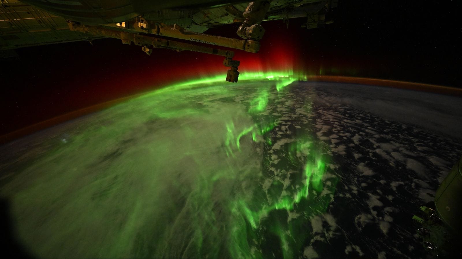
The altitude of the observation platform alters the interpretation of this process. Ground-based observers view the aurora through the dense, scattering lens of the lower atmosphere, obscuring the precise boundaries of particle precipitation. An orbital asset at an altitude of approximately 400 kilometers intersects the actual zone of excitation, providing a cross-sectional profile of the energy transfer.
The Tri-Color Atmospheric Spectrometry
The specific hues captured in orbital imagery are dictated by the quantum mechanics of electron precipitation. As accelerated solar electrons collide with ambient atmospheric constituents, they transfer kinetic energy, bumping atomic and molecular electrons into higher energy states. The subsequent relaxation of these states releases photons at fixed wavelengths.
ΔE = hν = hc / λ
Where:
- $ΔE$ is the energy difference between quantum states
- $h$ is Planck's constant
- $ν$ is the frequency of the emitted photon
- $c$ is the speed of light
- $λ$ is the resulting wavelength
Three distinct chemical boundaries dictate the structural anatomy of the Aurora Australis:
Atomic Oxygen Emissions (High Altitude)
At altitudes exceeding 200 kilometers, the atmospheric density is low enough that atomic oxygen dominates. A low-energy electron collision excites oxygen atoms to the $^1D$ state. Because this state has a long radiative lifetime (roughly 110 seconds), collisions with other particles can easily quench the energy before a photon escapes. However, at 400 kilometers, collisions are rare. The oxygen atoms successfully relax, emitting photons at a wavelength of 630.0 nanometers. This generates the deep red border seen at the highest altitudes of the auroral curtain.
Atomic Oxygen Emissions (Medium Altitude)
Between 100 and 200 kilometers, atmospheric density increases. Here, more energetic electron impacts excite oxygen to the $^1S$ state, which has a much shorter radiative lifetime of approximately 0.7 seconds. This rapid relaxation prevents quenching and yields a wavelength of 557.7 nanometers. This is the characteristic bright green hue that forms the primary body of most auroral displays.
Molecular Nitrogen Emissions (Low Altitude)
Below 100 kilometers, atomic oxygen becomes scarce, and molecular nitrogen ($N_2$) dominates the dense air. Extreme solar storms accelerate electrons with enough kinetic energy to penetrate to this depth. The ionization of $N_2$ produces a sharp emission spectrum at 427.8 nanometers (violet-blue) and structural transitions in neutral $N_2$ produce deep pinks and purples along the very bottom edge of the auroral curtain.
Orbital Geometries and Visual Distortion Factors
Capturing an aurora from LEO introduces significant observational variables that do not exist for ground-based astrophotography. The ISS travels at roughly 7.66 kilometers per second. At this velocity, time-exposure photography suffers from severe motion blur unless specific orbital mechanics are accounted for.
The primary optical challenge is line-of-sight velocity aberration. When a camera sensor faces forward relative to the orbital vector, the apparent motion of the aurora is radial, spreading outward from a central point. When looking perpendicular to the orbital track (nadir or limb views), the auroral features shear horizontally across the frame.
To counteract this, modern orbital documentation relies on high-sensitivity sensors capable of fast integration times (low exposure duration) coupled with high ISO values. This minimizes geometric smearing but introduces a secondary bottleneck: sensor noise. Space-based sensors are continuously bombarded by secondary cosmic rays and high-energy particles within the South Atlantic Anomaly (SAA). These particles manifest as hot pixels and transient white streaks, requiring sophisticated dark-frame subtraction algorithms to isolate the authentic auroral signal.
Furthermore, the perspective from 400 kilometers up alters the apparent scale of the phenomenon. Ground observers experience a localized, upward-looking view that emphasizes vertical curtain structures. Orbital observers look across the limb of the planet, viewing the aurora edge-on. This perspective amplifies the apparent brightness of the green and red layers due to path-length integration—the camera looks through a deeper physical volume of excited gas along the horizontal plane than it would looking straight up or down.
Systemic Risks to Space Architecture During High-Index Events
The solar flare that triggers a rare visual aurora also injects major operational risks into orbital infrastructure. A geomagnetic storm measured at a high Kp-index is not merely an aesthetic event; it represents a major destabilization of LEO environmental parameters.
The primary mechanical impact is atmospheric drag enhancement. The injection of solar particle energy heats the thermosphere, causing the upper atmosphere to expand outward. This increases the ambient particle density at the ISS operational altitude. The resulting drag accelerates orbital decay, requiring immediate or planned re-boost maneuvers using onboard propulsion systems to maintain structural velocity.
F_D = 0.5 * ρ * v^2 * C_D * A
Where:
- $F_D$ is the drag force
- $ρ$ is the atmospheric density (which escalates rapidly during solar storms)
- $v$ is the orbital velocity
- $C_D$ is the drag coefficient
- $A$ is the cross-sectional area of the spacecraft
The second vulnerability centers on spacecraft charging. The influx of high-energy electrons creates an uneven charge distribution across the exterior surfaces of an orbital asset. If the potential difference between non-conductive materials exceeds the dielectric breakdown threshold, an electrostatic discharge (ESD) occurs. These discharges can corrupt telemetry data, trigger false commands in flight computers, or degrade solar cell efficiency.
Operational Assessment of Auroral Tracking Data
To maximize the utility of orbital observation platforms during solar cycles, mission planning must transition from reactive capture to predictive scheduling. Relying on ground-based alerts creates a data lag that often misses the peak intensity of the auroral oval deformation.
Integrating real-time solar wind monitoring data from deep-space assets—such as the Deep Space Climate Observatory (DSCOVR) located at the Lagrangian Point 1 (L1)—allows for a 30- to 60-minute advance warning of CME arrivals. By tracking the exact orientation of the IMF IMF $B_z$ parameter and the velocity delta of the solar plasma, automated scheduling systems can align orbital cameras toward the southern auroral zone prior to the initial particle precipitation event. This predictive framework eliminates reliance on human response times, ensuring high-fidelity structural data is captured at the precise moment of maximum magnetospheric compression.